Geom Layer
Ming Chen
6/25/2017
Geom Layer
geom_abline, geom_hline and geom_vline
ggplot(data = mtcars) +
  geom_point(mapping = aes(x=0, y=5),
             stat = "identity",
             position = "identity",
             col = "red") +
  geom_abline(intercept = 5, slope = 2) +
  geom_hline(yintercept = 2.5, col = "blue") +
  geom_vline(xintercept = 5.0, col = "red") +
  geom_text(mapping = aes(x=2, y=5),
            stat = "identity",
            position = "identity",
            label = "intercept = 5, slop = 2") +
  geom_text(mapping = aes(x=2, y=1.5),
            stat = "identity",
            position = "identity",
            label = "yintercept = 2.5") +
  geom_text(mapping = aes(x=5.2, y=7.2),
            stat = "identity",
            position = "identity",
            label = "xintercept = 5.0",
            angle = 270) +
  coord_cartesian(xlim = c(0,10), ylim = c(0, 10)) +
  facet_grid(am~.)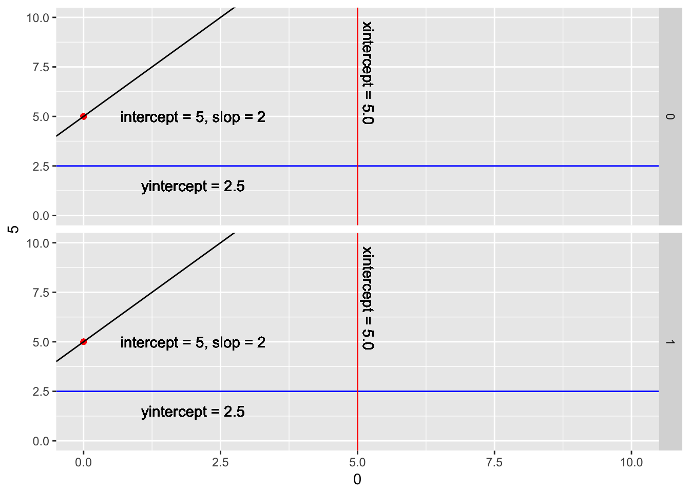
geom_bar and geom_col
geom_barusesstat_countto calculate the y values by default.geom_colusesstat_identityby default. You will need to provide theymapping.
ggplot(data = mpg) +
  geom_bar(mapping = aes(x=class, fill=factor(cyl)),
           position = position_stack()) +
  coord_flip()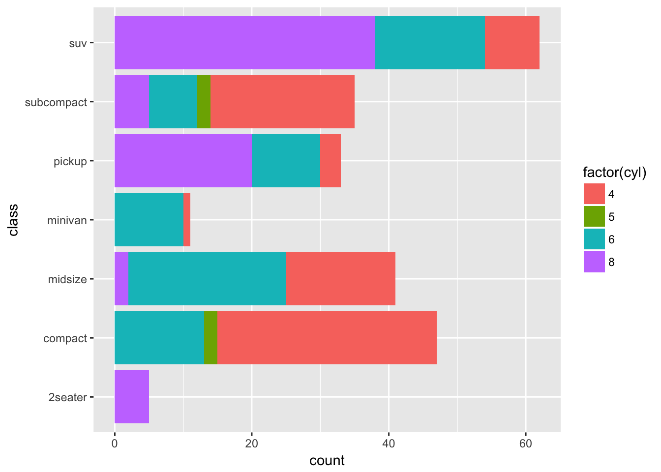
my_data = data.frame(x = rep(LETTERS[1:5], each=3),
                     y = sample(1:100, 15),
                     class = rep(letters[1:3], 5))
ggplot(data = my_data) +
  geom_col(mapping = aes(x=x, y=y, fill=class),
           position = position_stack()) +
  coord_flip()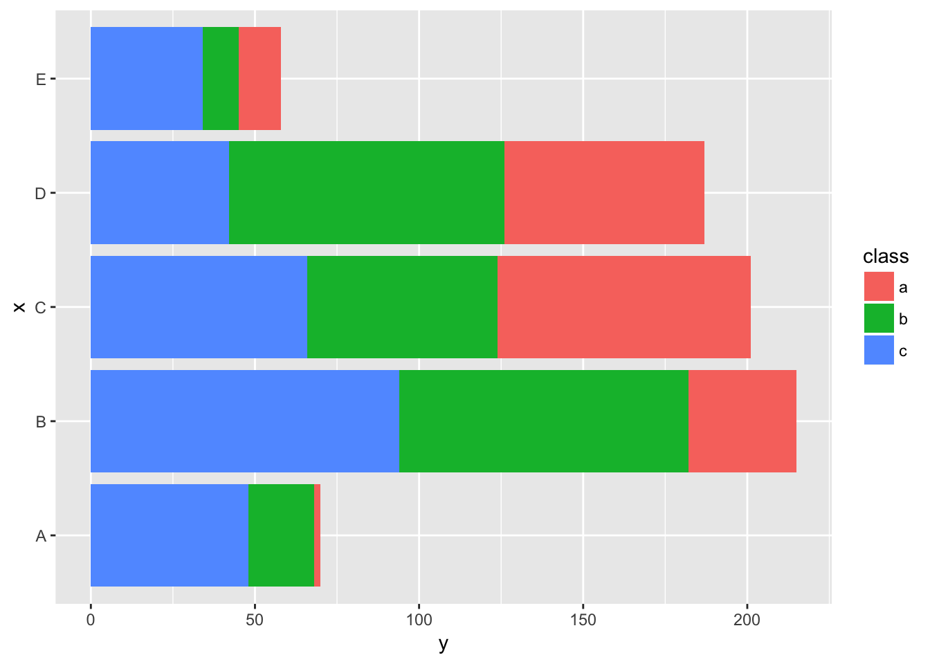
geom_bind2d
geom_bind2dmaps x, y and z to a coordinate system. z is the counts for each xy combination. If x and y are numeric, x and y are split into series of intervals (bin).
ggplot(data = mpg) +
  geom_bin2d(mapping = aes(x=manufacturer, y=displ)) +
  theme(axis.text.x = element_text(angle = 90))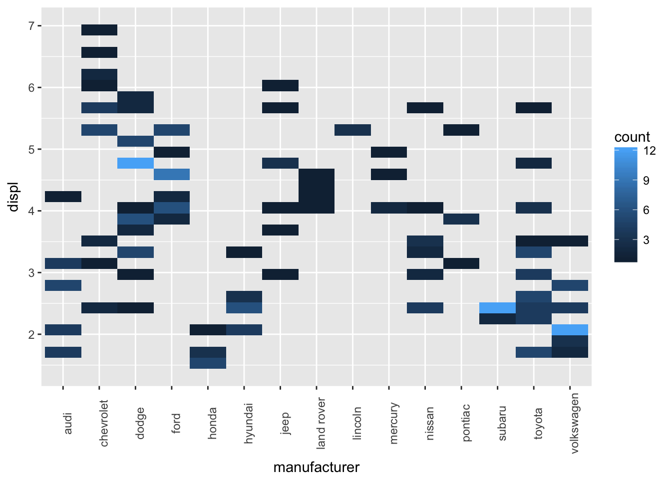
geom_boxplot
geom_boxplotusesstat_boxplotto convert y intolower,upper,middle,yminandymax.
ggplot(data = mpg) +
  geom_boxplot(mapping = aes(x=manufacturer, y=displ, fill=fl)) +
  theme(axis.text.x = element_text(angle = 90))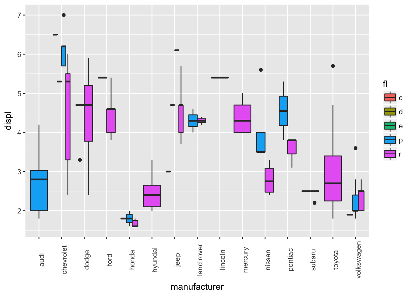
- Let’s see an example of using
stat_identity, which doesn’t transform the data.
my_data = data.frame(x = LETTERS[1:3],
                     ymin = sample(1:10,3),
                     lower = sample(11:20, 3),
                     middle = sample(21:30, 3),
                     upper = sample(31:40, 3),
                     ymax = sample(41:50, 3))
ggplot(data = my_data) +
  geom_boxplot(mapping = aes(x=x, ymin=ymin, lower=lower,
                             middle=middle, upper=upper, ymax=ymax),
               stat = "identity")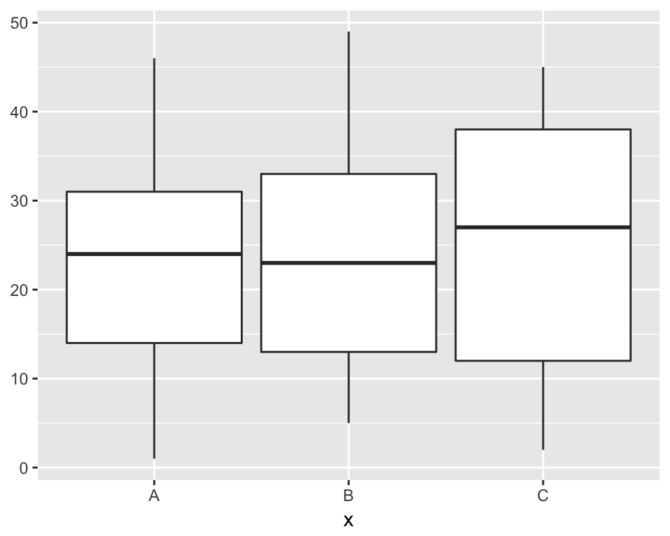
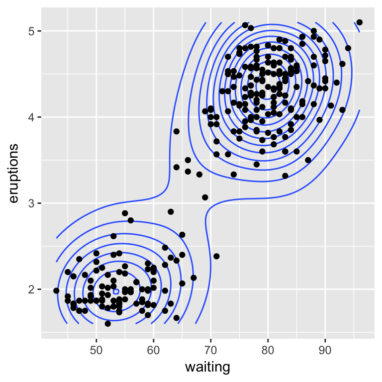
geom_density_2d
The 2d density is the density of a combination of (x, y). The density is estimated with the MASS::kde2d function. Points on the same contour line have the same existing probability of the estimated jointed distribution.
ggplot(data = faithful) +
  geom_density_2d(mapping = aes(x=waiting, y=eruptions),
                  stat = 'density_2d') +
  geom_point(mapping = aes(x=waiting, y=eruptions))